728x90
회귀 선을 정하기 위해서는 주어진 Y,X를 잘 설명할 수 있는 beta 혹은 theta 라고 쓰는 coefficent와 intercept에 대해서 잘 알아야 한다.
1. 단순 선형 회귀
우선 단순히 선형회귀를 하는 방법으로는
코드만 일부 첨부하자면
regr = linear_model.LinearRegression()
# fiiting
regr.fit(diabetes_X_train, diabetes_y_train.values)
# Make predictions on the training set
diabetes_y_train_pred = regr.predict(diabetes_X_train)
# The coefficients
print('Slope (theta1): \t', regr.coef_[0])
print('Intercept (theta0): \t', regr.intercept_)
Slope (theta1): 	 37.37884216052121
Intercept (theta0): 	 -797.0817390343262
이런 결과를 얻을 수 있다.
2. Normal Equation

3. Polynomial
차수를 올리게 되면 설명력이 높아진다. 다만 이럴 경우 오버피팅을 조심해야 한다

이런 경우가 overfitting에 해당한다. 너무 Train data set에만 집중하다가 생기는 모델의 오류라면 오류인 것이다.
다시, polynomial 로 predict하면
X_bmi = X_train.loc[:, ['bmi']]
X_bmi_p3 = pd.concat([X_bmi, X_bmi**2, X_bmi**3], axis=1)
X_bmi_p3.columns = ['bmi', 'bmi2', 'bmi3']
X_bmi_p3['one'] = 1
# Ordianry Least Squares
theta = np.linalg.inv(X_bmi_p3.T.dot(X_bmi_p3)).dot(X_bmi_p3.T).dot(y_train)
x_line = np.linspace(-0.1, 0.1, 10)
x_line_p3 = np.stack([x_line, x_line**2, x_line**3, np.ones(10,)], axis=1)
y_train_pred = x_line_p3.dot(theta)

# test

X_bmi_test =X_test.loc[:, ['bmi']]
X_bmi_p3_test = pd.concat([X_bmi_test, X_bmi_test**2, X_bmi_test**3], axis=1)
X_bmi_p3_test.columns = ['bmi', 'bmi2', 'bmi3']
X_bmi_p3_test['one'] = 1
다양한 방법으로 y_pred를 구했을 때를 비교한 표이다.

4. Ridge , Lasso Regularizaion
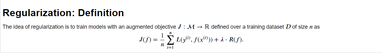
R(f)에 뭐가 들어가냐의 차이
Ridge L2 규제에서 theta 찾는 방법

held-out validation set에서 GridSearch나 Cross validation을 통해 lambda를 구할 수 있다.
Lasso L1 규제에서는 theta를 0으로 만드는 덜 중요한 feature를 고를 수 있어서 feature selector로서 쓰인다.

728x90
'IE & SWCON > Machine Learning' 카테고리의 다른 글
| SVM(Support Vector Machine) (1) | 2023.11.27 |
|---|---|
| 로지스틱 회귀를 사용한 클래스 확률 모델링 (1) | 2023.11.27 |
| [혼공머딥] chapter 6 - 교재 外 심화과정 (0) | 2023.08.30 |
| [혼공머딥] chapter 6 (0) | 2023.08.29 |
| [혼공머딥] chapter 5 (1) | 2023.08.22 |